Weibull Distribution | Reliability Analytics Blog

The Weibull distribution is particularly useful in reliability work since it is a general distribution which, by adjustment of the distribution parameters, can be made to model a wide range of life distribution characteristics of different classes of engineered items. One of the versions of the failure density function is

where
β is the shape parameter
η is the scale parameter or characteristic life (life at which 63.2% of the population will have failed)
Υ is the minimum life

In most practical reliability situations, Υ is often zero (failure assumed to start at t = 0) and the failure density function becomes

and the reliability and hazard functions become

Depending upon the value of β, the Weibull distribution function can take the form of the following distributions:

β < 1      Gamma
β = 1    Exponential
β = 2    Lognormal
β = 3.5 Normal (approximately)

Thus, it may be used to help identify other distributions from life data (backed up by goodness of fit tests) as well as being a distribution in its own right. Graphical and mathematical methods are used to analyze failure data and determine estimated for specific Weibull model parameters. One such tool is the Weibull analysis tool in the Reliability Analytics Toolkit.

Example Calculation

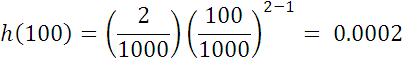
The failure times of a particular transmitting tube are found to be Weibull distributed with β = 2, and η = 1000 hours (consider η somewhat related to MTTF). Find the reliability of one of these tubes for a mission time of 100 hours, and the hazard rate after a tube has operated successfully for 100 hours.

Reliability Analytics Toolkit Example Weibull Calculation

Here we apply the Weibull Distribution from the Reliability Analytics Toolkit. For the first three inputs, highlighted in yellow, we enter the basic Weibull given in the problem statement. We select that we want three charts, f(t), R(t) and h(t) and the set the chart size to 400 pixels, smaller than the default size of 800. We override the default “time step division” and select a maximum value of 128, which provides for smoother plots (more plotted points), but takes more processing time. Finally, we a chart title, which is a prefix to the normal default chart titles.

Solution:

The reliability at 100 hours is 0.99, as represented by the green shaded area to the right of the 100 hour point in the probability density function (pdf) plot shown below. The unreliability, or probability of failure, is 0.01, as represented by the pink shaded area to the left of the 100 hour point in the pdf plot.

Reliability Analytics Toolkit Example Weibull Analysis

A related tool is the Weibull Analysis tool from the Reliability Analytics Toolkit. In the above examples, the the Weibull shape parameter (β) and characteristic life parameter (η) were given as part of the problem statement. What if you do not know these? There are databases published with estimates for different types equipment; however, a more fundamental method is to do a Weibull analysis on specific time-to-failure data for the specific item in question. The Weibull analysis results then provide equipment-specific estimates for the shape parameter and characteristic life.

The picture below shows example input data highlighted in yellow (select test set 3 under the options to duplicate this example). The data input format (time-to-failure, box 1 in the picture below) is a failure time followed by either an “f” or an “s”, indicating a failure or suspension (i.e., item did not fail), one record per line. For this example, we are selecting that we want to generate plots and would also like to generate Weibull f(t), F(t), R(t) and h(t) equations containing the numerical parameters found from analyzing the time-to-failure input data. The tool generates both report quality equations and Microsoft Excel based equations that can be copied and pasted into Excel for use in other analyses.

The above input results in the following output estimates for parameters associated graphs and parameter-specific equations.

Solution:
Location parameter, failure free life (δ): 0.00
Parameter estimates based on linear regression: Shape parameter (β): 3.34
Characteristic life (η): 190.30
Correlation coefficient (R²): 0.96
Mean life (μ): 170.79
Variance (σ²): 3,188.99

Parameter estimates based on maximum likelihood estimation (MLE):

Mean life (μ): 181.38
Variance (σ²): 4,432.37

Failure time values are adjusted (i.e., they represent moving failure points left or right until they intersect the best fit straight line in the Weibull Probability Plot shown above.).